Ergodicity and Stationarity. Luck but Not for You
We are constantly making decisions under uncertainty where information is limited and the outcome of the decision is not granted. You don’t know if your startup investment will go to zero. You don’t know if a given health treatment will save your life. You don’t know if you will win a hand in poker.
Luckily, statistics help us to manage uncertainty. Metrics such as mean, median, mode or percentiles give us information about the past. We can incorporate these metrics in our decision making process to trade-off the risk and reward.
The problem. Most people apply statistics wrongly in their decision making process. In this post we will explain the concepts of ergodicity and stationarity exemplified with three use cases:
- The Ergodic Coin Flip
- The Non-Ergodic Bet
- The Non-Stationary Cookie Baking
All real-life use cases that can be modeled as stochastic processes are never ergodic nor stationary. Yet people keep applying statistics as if they were.
Here you will learn what happens if you do so, and how to identify such situations.
The Ergodic Coin Flip
Ergodicity is a well-known concept in statistics. It’s a property of stochastic processes. If you observe a single system over a long period and give the same statistical properties as observing many systems at a single point in time, we say that it is ergodic.
A coin flip of an unbiased coin is an ergodic process. If 10000 people flip a coin once or 1 person flips a coin 10000 times, both stochastic processes will have the same properties. For example, the expected value of heads and tails will be 50:50. Since it is ergodic, you as an individual will get 50:50 heads/tails if we consider enough flips.
A fancy way of saying that one coin flip over n trials is the same a flipping n coins once can be expressed as follows:
We call the term on the left the time average. This is a single person flipping the coin multiple times. The one on the right is the ensemble average, which is multiple people flipping a coin once.
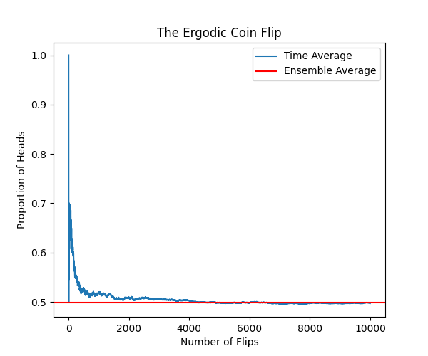
Let’s model the coin flip with Python, using a Bernoulli process, where the odds of success are always 0.5.
Collapse Code Expand Code
 1import numpy as np
 2import matplotlib.pyplot as plt
 3
 4def coin_flip():
 5    return np.random.choice(['H', 'T'])
 6
 7def avg(flips):
 8    return flips.count('H') / len(flips)
 9
10n_flips = 10000
11n_coins = 10000
12single_sequence_flips = [coin_flip() for _ in range(n_flips)]
13all_sequences_flips = [coin_flip() for _ in range(n_coins)]
14
15time_avg = [avg(single_sequence_flips[:i + 1]) for i in range(n_flips)]
16ensemble_avg = avg(all_sequences_flips)
17
18def plot_averages(time_averages, ensemble_average, n_flips):
19    plt.figure(figsize=(6, 5))
20    plt.plot(range(n_flips), time_averages, label='Time Average')
21    plt.axhline(y=ensemble_average, color='r', linestyle='-', label='Ensemble Average')
22    plt.xlabel('Number of Flips')
23    plt.ylabel('Proportion of Heads')
24    plt.title('The Ergodic Coin Flip')
25    plt.legend()
26    plt.show()
27
28plot_averages(time_avg, ensemble_avg, n_flips)
With 10.000 trials we observe that both time average of a single person flipping the coin and the ensemble average of multiple people flipping a coin once match. We say it is ergodic. It is important to note that with just a few flips, you may not get 50:50 heads/tais. But statistics guarantee you that the more flips you do, the closer you will get to that.
The bad news. Nothing in real life is ergodic. Not even a coin flip. All coins are slightly biased. With every flip, the coin will wear down slightly, potentially altering its bias. External factors like wind or temperature will further worsen the result. Not only is it non-ergodic but also non-stationary.
The Non-Ergodic Bet
Think of the following bet. You start with 1000€ and flip a coin multiple times, betting in each round all your wealth. If heads, you earn +80%. If tails, you lose -50%.
It may sound like a good bet. Spoiler, it is not. With statistics, we can calculate the expected value for each bet. That’s 0.5*0.8 - 0.5*0.5 = 15%, meaning that 15% is earned on average on each bet.
After 20 bets the average would be +15% per bet, or 1000*(1 + 0.15)^20. That’s 16366€, which seems like a good deal, meaning that on average the expected wealth after the 20 bets is that. Why not play that game?
The problem is that we have calculated the expected wealth for the so-called ensemble. The ensemble average. In other words, that’s what infinite players will get playing after 20 bets. You are not the ensemble. You are an individual.
This stochastic process is not ergodic, since the ensemble doesn’t match individual wealth paths. Let’s model this with Python and check that.
Collapse Code Expand Code
 1import matplotlib.pyplot as plt
 2import numpy as np
 3from scipy import stats
 4
 5def simulate_gambler(initial_wealth, p_win, return_win, return_lose, n_bets):
 6    wealth = [initial_wealth]
 7    for _ in range(n_bets):
 8        if np.random.choice(['Head', 'Tails'], p=[p_win, 1-p_win]) == 'Head':
 9            wealth.append(wealth[-1] * (1 + return_win))
10        else:
11            wealth.append(wealth[-1] * (1 + return_lose))
12    return wealth
13
14
15def plot_wealth(wealth_paths):
16    plt.figure(figsize=(6, 5))
17    for i, array in enumerate(wealth_paths):
18        if i == 0:
19            plt.plot(array, linestyle='--', color='red', linewidth=1, label='Individuals')
20        else:
21            plt.plot(array, linestyle='--', color='red', linewidth=1)
22    ensemble_avg = np.mean(wealth_paths, axis=0)
23    plt.plot(ensemble_avg, linewidth=2, label='Ensemble Average')
24    plt.text(len(ensemble_avg)+1, ensemble_avg[-1],  f'{round(ensemble_avg[-1])}',
25             bbox=dict(facecolor='white', edgecolor='black', boxstyle='round,pad=0.5'),
26             fontsize=12, ha='right')
27    plt.xlabel('Number of Bets')
28    plt.ylabel('Wealth (€)')
29    plt.title('The Non-Ergodic Bet')
30    plt.yscale('log')
31    plt.legend()
32    plt.show()
33
34def plot_cdf(multiple_gamblers):
35    plt.figure(figsize=(6, 5))
36    sorted_data = np.sort([i[-1] for i in multiple_gamblers])
37    cdf = np.arange(1, len(sorted_data) + 1) / len(sorted_data) * 100
38    plt.plot(sorted_data, cdf, linestyle='-', marker='', color='b')
39    plt.xscale('log')
40    plt.title('Wealth CDF')
41    plt.xlabel('Wealth (€)')
42    plt.ylabel('Cumulative Wealth (%)')
43    plt.grid(True)
44
45initial_wealth = 1000  # Initial wealth
46p_win = 0.5            # Probability of winning
47return_win = +0.80     # +80% if win
48return_lose = -0.5     # -50% if lose
49n_bets = 20
50
51multiple_gamblers = [simulate_gambler(initial_wealth, p_win, return_win, return_lose, n_bets) for _ in range(100000)]
52
53print(f"Mean (€): {np.mean(multiple_gamblers, axis=0)[-1]:.0f}", )
54print(f"Mode (€): {stats.mode(multiple_gamblers, axis=0).mode[-1]:.0f}")
55print(f"Losers (%): {np.mean(np.array(multiple_gamblers)[:, -1] < 1000) * 100:.0f}")
56
57plot_cdf(multiple_gamblers)
58plot_wealth(multiple_gamblers)
We will use the following configuration. Unbiased coin with +80% wealth increment on heads and -50% decrement on tails. Simulate 20 bets for 100000 players.
1initial_wealth = 1000  # Initial wealth
2p_win = 0.5            # Probability of winning
3return_win = +0.80     # +80% if win
4return_lose = -0.5     # -50% if lose
5n_bets = 20
As expected, the average (called ensemble average) of all players after 20 bets is 16 399 which is pretty close to the calculated number.
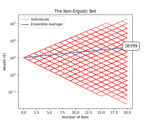
But check the red paths. These are the wealth that individual users will get over each bet. As you can see, some end up with a wealth way higher than the average, but most of them end up worse close to bankrupt.
The mean is a rather bad metric. You can see that the mode, which is the most frequent value in the dataset, is 349 €. In other words, most of the gamblers have lost money, 59%.
1Mean (€): 16399
2Mode (€): 349
3Losers (%): 59
Yes you can be lucky. One lucky player got to >10 000 000 € but that was luck. Among all 100000 players, the chances that you end up losing are rather high.
Here is the common mistake people make. They see an average and think that they, as individuals will get just that. No you won’t. It’s non-ergodic, you can’t do that.
A similar example can be simulated with different odds and returns. In this case we have 90% of probability of winning +80% but if you lose, you go bankrupt.
1initial_wealth = 1000  # Initial wealth
2p_win = 0.9            # Probability of winning
3return_win = +0.80     # +80 % if win
4return_lose = -1       # Bankrupt
5n_bets = 20
This case is more of a binary situation. Lucky players get more and more wealth, but at some point, all go bust. Around 88% of the players lose money in this simulation.
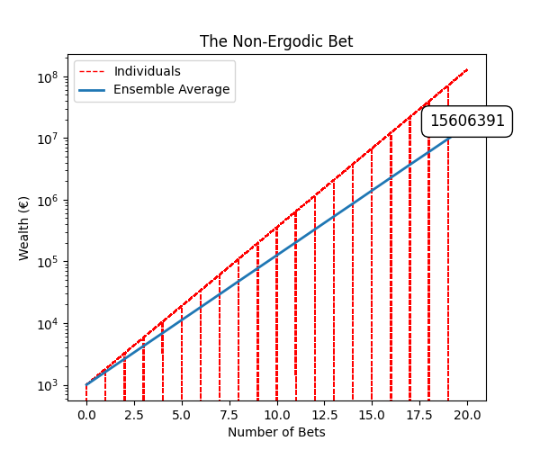
1Mean (€): 15606391
2Mode (€): 0
3Losers (%): 88
This case is even worse, since once you go bust, you can’t keep playing. You are out of the game. The ensemble average doesn’t account for that. Once you go bust, you don’t care anymore about the ensemble average, since you are out.
As a note, there is an optimal strategy for these kinds of sequential bets, which is the Kelly Criterion. It recommends not betting on everything all the time, but keeping a given percent.
The Non-Stationary Cookie Baking
Now let’s talk about stationarity. We say a process is stationary if its statistical properties, such as mean, variance, and autocorrelation, are constant over time. Depending on a few things beyond the post, there is strict or weak stationarity.
Ergodicity and stationarity are related. If a process is not stationary, most likely it won’t be ergodic. For example, having bursts of random wind during a coin flip will make it non-ergodic and non-stationary.
Let’s say you are baking cookies in the oven. Your oven can’t keep the temperature at exactly 200º all the time. In the upper tray, only 190º are reached. Your kid may open the door during a batch. An unexpected power outage may last for few minutes.
All this makes cookie baking a non-stationary stochastic process. The cookies of the first batch may experience a different average temperature than the second batch. 95% of the first batch of cookies may be perfect, but only 92% in the second batch.
Moreover, it’s also non-ergodic. You won’t get the same amount of perfect cookies if you bake 10 in 1 batch or 1 each batch during 10 batches.
Summary
- It is of paramount importance to identify when we are using statistics in non-ergodic non-stationary processes. Think twice to avoid surprises.
- Most of the averages you are presented are ensemble averages. They won’t apply to you as an individual if the process is non-ergodic.
- Investment strategies like DCA are a way to get closer to the ensemble average on financial markets, which are non-ergodic non-stationary.
- In venture capital, the success rate of startups is very low, 10-20%. But again, this is an ensemble average of a non-stationary process. A downturn in the markets may lower this. The more startups and the wider the time window, the closer you will get to the ensemble.