Convolutions, Fast Fourier Transform and Polynomials

You may remember from high school what a polynomial is. If so, you may also remember how to multiply two of them. But what if I told you that the method you were taught is slow as F?

In this post we will connect polynomials with the Fourier Transform and convolutions, and show you how to multiply polynomials with $O(nlogn)$ complexity instead of $O(n^2)$, being the latter the method that’s taught in high school.

Polynomials: A Quick Recap

Let's do a quick recap on what polynomials are. Formally defined, a polynomial $P(x)$ is a sum of terms where each one is an indeterminate variable $x$ with some exponent $k$ multiplied by a coefficient $a_k$.

This is an example of a polynomial. Note that we say it has a degree $2$ since it is its maximum exponent. It can be expressed as a vector like [5, 2, 9] or [9, 2, 5] depending on the notation we use.

Let $P(x)$ and $Q(x)$ be two polynomials, we can perform different operations with them, like adding or subtracting them. In both cases, the result is trivially computed by summing (or subtracting) each term individually. In Python, we can compute the result as follows. Note that this works with p and q having the same degree. You can use zip_longest for different degrees.

# a + b
[a + b for a, b in zip(p, q)]

# a - b
[a - b for a, b in zip(p, q)]

On the other hand, we can also multiply them. And here is where things get interesting. Multiplying $Y(x) = P(x) * Q(x)$ is a bit more complex than adding or subtracting. Let’s see an example:

As you can see, we have a bunch of multiplications here. And well, the higher the degree of $P(x)$ and $Q(x)$ the more multiplications we will have. More specifically, the complexity is $O(n^2)$ which is not good. Can we do it better?

Convolutions

Before answering the question if we can do better than $O(n^2)$ to multiply polynomials, let's introduce the concept of convolution, since it will come in handy to understand what’s next.

Convolution is defined both in continuous and discrete domains. The continuous domain might be cool for mathematicians, but we engineers who do real things prefer the discrete domain. We can define the convolution in the discrete domain of two discrete signals $p$ and $q$ as:

The operation is rather simple. You just need to flip $q$ and sum the product of all elements that overlap with $p$. Trust me, it's easier than it looks. Let's say we have two discrete signals p and q represented as vectors:

p = [2, 3, 4]
q = [5, 6, 7]

Let's calculate the convolution of both $p * q$. Note that $*$ here is the convolution of both signals. We just need to flip q and move it from left to right until we are done. Note that we don’t have to do it from $-\infty$ to $+\infty$ since we have a discrete signal of just 3 samples. The maths are not difficult but lets try to visualize it step by step.

Then we move the flipped version of q one element to the right.

And one more.

And one more.

And one last more.

Each element represents a value of our new signal y which is p * q. We can see that it has a total length of 5 elements. We can express y as follows:

y = [10, 27, 52, 45, 28]

If you remember $Y(x)$ from the previous section, you will have noticed that its the same. The p and q we’ve just used are the vector representations of $P(x)$ and $Q(x)$. As a reminder this is $Y(x)$ from before:

So multiplying two polynomials can be expressed as a convolution. As you can see, the result is the same. Both using the convolution and the polynomial multiplication method seen above, which most likely you studied in high school.

In the next section, you will understand why convolutions are cool, and how the FFT can help us to multiply polynomials faster.

Fourier Transform, and the FFT

The Fourier Transform is a very powerful transformation that allows converting a signal from time domain to frequency domain. It's some kind of base change, where instead of looking at the signal from a time perspective, we look at it from a frequency point of view.

Instead of saying that the signal has $x_1$ value at $t_1$ time, and $x_2$ at $t_2$, etc, we say that the signal is made of different oscillating frequencies at different rates. These oscillating frequencies are represented with sines and cosines and have a coefficient and a phase attached to them. Every signal that you can imagine, can be expressed as the sum of sines and cosines. The only problem is to know which sines/cosines represent that signal.

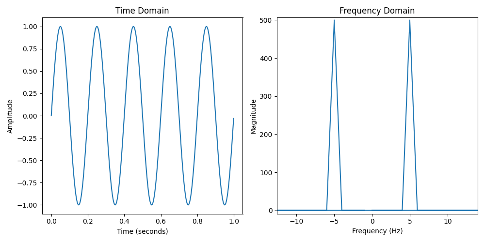
Let's see the simplest example. Imagine a pure sinusoidal signal of frequency 5 Hz.

import numpy as np
import matplotlib.pyplot as plt

fs = 1000  # Sampling frequency (Hz)
t_end = 1  # Duration in seconds
f0 = 5     # Frequency of the sine wave (Hz)

t = np.linspace(0, t_end, int(fs * t_end), endpoint=False)
y = np.sin(2 * np.pi * f0 * t)
Y = np.fft.fft(y)
freq = np.fft.fftfreq(len(y), d=1/fs)

If we take the FFT of this signal, it will look as follows in the frequency domain.

# Prepare the figure and axes
fig, (ax1, ax2) = plt.subplots(1, 2, figsize=(10, 5))

# Plot the sine wave
ax1.plot(t, y, label=f'Sine Wave {f0} Hz')
ax1.set_title('Time Domain')
ax1.set_xlabel('Time (seconds)')
ax1.set_ylabel('Amplitude')

# Plot the magnitude of the Fourier Transform
ax2.plot(freq, np.abs(Y), label='Magnitude of FFT')
ax2.set_title('Frequency Domain')
ax2.set_xlabel('Frequency (Hz)')
ax2.set_ylabel('Magnitude')

plt.tight_layout()
plt.show()

In the frequency domain, it looks like a delta, exactly at the frequency 5. This means that the signal on the left side (time domain) can be expressed as one sinus with frequency 5. Different ways of referring to the same signal.

Before continuing, let's clarify the concepts. They all refer to the same thing but have some minor differences:

• Fourier Transform (FT): Fourier Transform defined in continuous domain.
• Discrete Fourier Transform (DFT): Fourier Transform defined for discrete signals. In practice, this is what matters, since nowadays all signals are digital, hence discrete.
• Fast Fourier Transform (FFT): It is an algorithm that allows to compute the Discrete Fourier Transform efficiently, $O(nlogn)$ instead of $O(n^2)$.

Finally, let me introduce you to the equation you have been waiting for. The Discrete Fourier Transform.

It takes a discrete signal in time domain $x[n]$ and converts it to the frequency domain $X[k]$. Note that what it does is quite simple. Each sample of $X[k] is calculated by taking each sample of $x$ and multiplying it with a complex number, that represents a given frequency.

It's some kind of projection, where each element of the input signal is projected into sines, and then added up together. But let's go back to the main goal of this post. We wanted to multiply polynomials faster.

One of the advantages of the DFT and working in the frequency domain, is that it converts a convolution into a simple multiplication. In other words, performing the convolution of two signals in time domain is equivalent to multiplying them in the frequency domain.

And as you can imagine, multiplication is way faster than convolution. But we are still missing one piece. In order to benefit from this, we have to convert first from time domain to frequency domain. And well, this takes time.

The good news is that the FFT allows us to convert from $x[n]$ (time domain) to $X[k]$ (frequency domain) with $O(nlogn)$ complexity.

Multiplying Polynomials Faster

As a quick recap, the way to multiply polynomials that you learned in high school is very inefficient and has a $O(n^2)$ complexity, where $n$ is the degree of the polynomials. This means that multiplying two polynomials or order 100 is way way more difficult than order 20. This doesn’t scale for huge polynomials. But we have an alternative:

• Convert our polynomials to frequency domain. Complexity $O(nlogn)$ using the FFT.
• Multiply them, which is cheaper than convolution. Complexity $O(n)$, simple element-wise multiplication.
• Convert the resulting polynomial back to time domain. Complexity $O(nlogn)$ using the IFFT.

It may seem like a lot of operations, but for large polynomials this is way faster than the naive method that you were taught in high school. Let's see an example in Python and benchmark both approaches.

Let's define multiply_naive which multiplies polynomials as you were taught in high school with $O(n^2)$ complexity.

import numpy as np
import random
import timeit
import matplotlib.pyplot as plt

def multiply_naive(p, q):
    result_size = len(p) + len(q) - 1
    result = [0] * result_size
    for i in range(len(p)):
        for j in range(len(q)):
            result[i + j] += p[i] * q[j]

    return result

And multiply_fft which uses the FFT/IFFT and does a multiplication in the frequency domain, with $O(nlogn)$ complexity.

def multiply_fft(p, q):
    length = 2 ** np.ceil(np.log2(len(p) + len(q) - 1)).astype(int)
    f_padded = np.pad(p, (0, length - len(p)))
    g_padded = np.pad(p2, (0, length - len(q)))

    # Calculate FFT and multiply
    Y = np.fft.fft(f_padded) * np.fft.fft(g_padded)

    result_coefficients = np.round(np.fft.ifft(Y).real).astype(int)
    return np.trim_zeros(result_coefficients, 'b').tolist()

If we multiply the previous polynomials p and q, we can see how the result is the same as before.

p = [2, 3, 4]
q = [5, 6, 7]

print(multiply_fft(p, q))
print(multiply_naive(p, q))

# [10, 27, 52, 45, 28]
# [10, 27, 52, 45, 28]

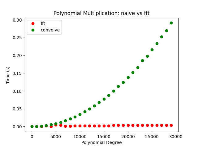
However, these polynomials have a low degree. Let's try to multiply polynomials up to degree 500 and see the time it takes using each method. We can do so with the following snippet:

n_runs = 10
tiempos_naive, tiempos_fft = [], []
for grado in range(1, 500, 10):
    p = [random.randint(1, 100) for i in range(grado)]
    q = [random.randint(1, 100) for i in range(grado)]

    tiempos_naive.append(timeit.timeit('multiply_naive(p, q)', number=n_runs, globals=globals())/n_runs)
    tiempos_fft.append(timeit.timeit('multiply_fft(p, q)', number=n_runs, globals=globals())/n_runs)

plt.plot(tiempos_naive, 'bo', label="naive")
plt.plot(tiempos_fft, 'ro', label="fft")
plt.title("Polynomial Multiplication: naive vs fft")
plt.ylabel("Time (s)")
plt.xlabel("Polynomial Degree")
plt.legend()
plt.show()

And we get the following times. As you can see, for low-degree polynomials it may not make sense to use the FFT approach, since the FFT/IFFT back-and-forth conversions take more time than the naive approach. However, as the degree increases, we can observe how the FFT approach is way more efficient.

Summary

Let’s summarise what we have seen:

• Multiplying polynomials using the naive method has $O(n^2)$ complexity.
• Polynomial multiplication can be seen as a convolution.
• A convolution in time domain is equivalent to a simple multiplication in frequency domain.
• We can convert polynomials to frequency domain with $O(nlogn)$ complexity using the FFT.
• Adding all together, we can multiply polynomials in frequency domain in $O(nlogn)$ which is faster than what you were taught in high school.